Take-home_Ex2

Author

Low Ji Xiong

Introduction

The success of Singapore’s public transport is commonly recognised as 1 of the quintessential indicator of its rapid growth and prosperity since her independence in 1965. It comprises of both public buses as well as mass rapid transport (MRT) trains. While the MRT network has been expanding across the many zones within Singapore, the bus network remains the most option accessible and reliable option amongst the two.

Thus, the utilisation pattern of buses are of key importance to multiple aspects of Singapore’s socio-economic spheres, ranging from areas of work productivity and efficiency, environmental impact, tourism, and even to potential impact to cost of living and real estate development; which underpins the impetus of this exercise to gain a better understanding of the utilisation patterns and characteristics of Singapore’s bus stops.

Objectives

The key objectives of this exercise are:

To perform geovisualisation and analysis of Origin-Destination flows of passenger trips
To perform Spatial Interaction Modelling for Origin-Destination flows of passenger trips

Getting Started

The code chunk below load the following packages:

tmap: for thematic mapping
sf: for simple feature geospatial data handling
sp: for spatial polygon geospatial data handling
tidyverse: for non-spatial data handling.
knitr: for creating html table
reshape2: for reshaping functions
stplanr:
spdep:
sfdep: for creating an sf and tidyverse friendly interface as well as for introducing new functionality that is not present in spdep
plotly: for interactive plots

pacman::p_load(tmap, sf, sp, tidyverse, knitr,  reshape2, stplanr) # plotly, zoo, Kendall,sfdep,spdep,

Importing and preparing the Base Geospatial and Aspatial Data

Aspatial data

Firstly, the data set Passenger Volume by Origin Destination Bus Stops for the month of October 2023 from LTA DataMall, will be imported by using ‘read_csv()’ of **readr* package.

odbus <- read.csv("data/aspatial/origin_destination_bus_202310.csv")

Glimpse function is then used to discover the data type of the variables in the dataset.

glimpse(odbus)

Rows: 5,694,297
Columns: 7
$ YEAR_MONTH          <chr> "2023-10", "2023-10", "2023-10", "2023-10", "2023-…
$ DAY_TYPE            <chr> "WEEKENDS/HOLIDAY", "WEEKDAY", "WEEKENDS/HOLIDAY",…
$ TIME_PER_HOUR       <int> 16, 16, 14, 14, 17, 17, 17, 7, 14, 14, 10, 20, 20,…
$ PT_TYPE             <chr> "BUS", "BUS", "BUS", "BUS", "BUS", "BUS", "BUS", "…
$ ORIGIN_PT_CODE      <int> 4168, 4168, 80119, 80119, 44069, 20281, 20281, 190…
$ DESTINATION_PT_CODE <int> 10051, 10051, 90079, 90079, 17229, 20141, 20141, 1…
$ TOTAL_TRIPS         <int> 3, 5, 3, 5, 4, 1, 24, 2, 1, 7, 3, 2, 5, 1, 1, 1, 1…

From above, the values in ORIGIN_PT_CODE and DESTINATON_PT_CODE in the odbus tibble data frame are in numeric data type.

Using appropriate tidyverse functions, these data values will be converted into factor data type.

odbus$ORIGIN_PT_CODE <- as.factor(odbus$ORIGIN_PT_CODE)
odbus$DESTINATION_PT_CODE <- as.factor(odbus$DESTINATION_PT_CODE)

Using Glimpse once more to check, the values in ORIGIN_PT_CODE and DESTINATON_PT_CODE odbus in the tibble data frame are now in factor data type, as below.

glimpse(odbus)

Rows: 5,694,297
Columns: 7
$ YEAR_MONTH          <chr> "2023-10", "2023-10", "2023-10", "2023-10", "2023-…
$ DAY_TYPE            <chr> "WEEKENDS/HOLIDAY", "WEEKDAY", "WEEKENDS/HOLIDAY",…
$ TIME_PER_HOUR       <int> 16, 16, 14, 14, 17, 17, 17, 7, 14, 14, 10, 20, 20,…
$ PT_TYPE             <chr> "BUS", "BUS", "BUS", "BUS", "BUS", "BUS", "BUS", "…
$ ORIGIN_PT_CODE      <fct> 4168, 4168, 80119, 80119, 44069, 20281, 20281, 190…
$ DESTINATION_PT_CODE <fct> 10051, 10051, 90079, 90079, 17229, 20141, 20141, 1…
$ TOTAL_TRIPS         <int> 3, 5, 3, 5, 4, 1, 24, 2, 1, 7, 3, 2, 5, 1, 1, 1, 1…

Geospatial data

The geospatial data for BusStop downloaded from LTA DataMall into RStudio is then imported and saved as a sf data frame named busstop. Projected coordinate system is selected, which tends to be more accurate for distance measurement.

busstop <- st_read(dsn = "data/geospatial",
                   layer = "BusStop") %>%
  st_transform(crs = 3414)

Reading layer `BusStop' from data source 
  `C:\jayexx\ISSS624\Take_home_Exercises\Take_home_Ex2\data\geospatial' 
  using driver `ESRI Shapefile'
Simple feature collection with 5161 features and 3 fields
Geometry type: POINT
Dimension:     XY
Bounding box:  xmin: 3970.122 ymin: 26482.1 xmax: 48284.56 ymax: 52983.82
Projected CRS: SVY21

Using the glimpse() function, the structure of busstop sf tibble data frame is as follows.

glimpse(busstop)

Rows: 5,161
Columns: 4
$ BUS_STOP_N <chr> "22069", "32071", "44331", "96081", "11561", "66191", "2338…
$ BUS_ROOF_N <chr> "B06", "B23", "B01", "B05", "B05", "B03", "B02A", "B02", "B…
$ LOC_DESC   <chr> "OPP CEVA LOGISTICS", "AFT TRACK 13", "BLK 239", "GRACE IND…
$ geometry   <POINT [m]> POINT (13576.31 32883.65), POINT (13228.59 44206.38),…

The geospatial data for the Singapore Master Plan Subzone 2019 data downloaded from data.gov.sg is also imported and save it as a sf data frame named mpsz, similarly in projected coordinate system.

mpsz <- st_read(dsn = "data/geospatial",layer ="MPSZ-2019") %>%
  st_transform(crs = 3414)

Reading layer `MPSZ-2019' from data source 
  `C:\jayexx\ISSS624\Take_home_Exercises\Take_home_Ex2\data\geospatial' 
  using driver `ESRI Shapefile'
Simple feature collection with 332 features and 6 fields
Geometry type: MULTIPOLYGON
Dimension:     XY
Bounding box:  xmin: 103.6057 ymin: 1.158699 xmax: 104.0885 ymax: 1.470775
Geodetic CRS:  WGS 84

Preparing Hexagonal Grid for Traffic Analysis Zone (TAZ)

Creating hexagonal grid in sf format with grid_id as follows.

hxgn_grid = st_make_grid(mpsz, c(375, 375), what = "polygons", square = FALSE)

# To sf and add grid ID
hxgn_grid_sf = st_sf(hxgn_grid) %>%
  mutate(grid_id = 1:length(lengths(hxgn_grid)))

In the above, the hexagonal grid size is chosen to be 375m by 375m is based on the assumption that the maximum willingness of an average commuter to walk being 375m*2 which is 750m.

Merging Hexagonal Grid with Busstop Geospatial data

Imported busstop data is merged with Hexagonal grid as follows.

busstop_hxgn_grid <- st_intersection(busstop, hxgn_grid_sf) %>%
  select(BUS_STOP_N, grid_id) %>%
  st_drop_geometry()

Warning: attribute variables are assumed to be spatially constant throughout
all geometries

Check for BUS_STOP_N with duplicate grid_id is then performed as follows.

check_duplicate <- busstop_hxgn_grid %>%
  group_by(BUS_STOP_N) %>%
  summarise(num_grid_id = n_distinct(grid_id))

From the resultant table in the code above, out of 5,144 busstops, 4 intercept across 2 grid_id.

Hence, for this exercise, to avoid double counting of trips subsequently, the duplicate grid_id for the 4 busstops are removed.

busstop_hxgn_grid <- distinct(busstop_hxgn_grid, BUS_STOP_N, .keep_all = TRUE)

busstop_hxgn_grid data is re-merged with sf tibble data and converted to sf object class for subsequent geo-visualisation of hexagon grid for all busstops in Singapore, named as busstop_hxgn_grid_sf.

busstop_hxgn_grid_sf <- left_join(busstop_hxgn_grid, 
                           hxgn_grid_sf,
                           by = c("grid_id" = "grid_id"))%>%
  select(BUS_STOP_N, grid_id, hxgn_grid) %>%
  st_sf()

tm_shape(busstop_hxgn_grid_sf) + 
  tm_polygons()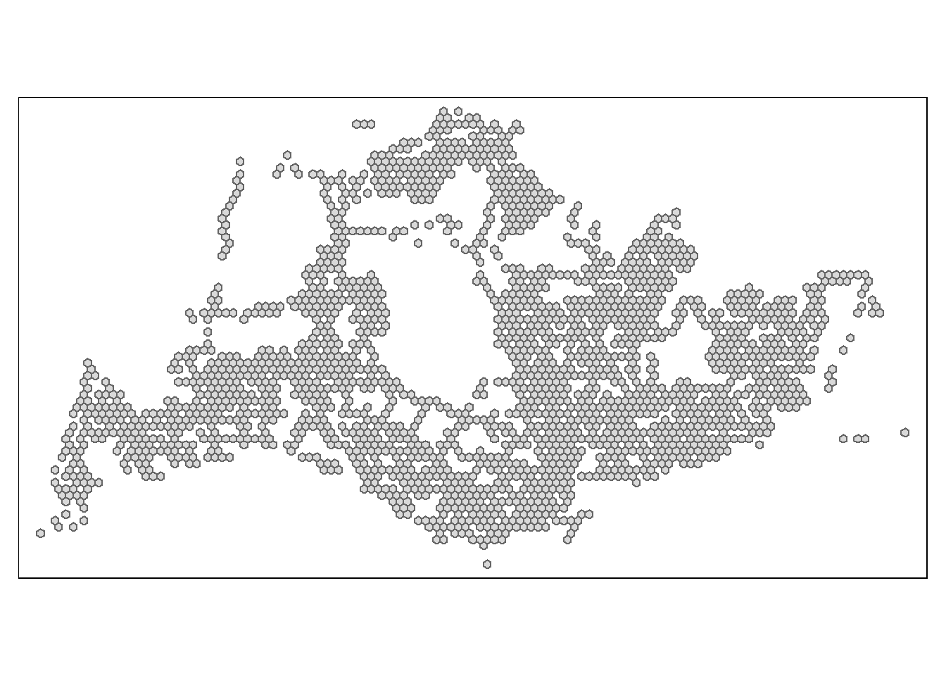

Extracting the passenger trips for Weekday Evening Peakhour

For the purpose of this exercise, extract commuting flows during weekday evening peak and label the output tibble data table as odbus_wkd17_20.

odbus_wkd17_20 <- odbus %>%
  filter(DAY_TYPE == "WEEKDAY") %>%
  filter(TIME_PER_HOUR >= 17 &
           TIME_PER_HOUR <= 20) %>%
  group_by(ORIGIN_PT_CODE,
           DESTINATION_PT_CODE) %>%
  summarise(TRIPS = sum(TOTAL_TRIPS))

`summarise()` has grouped output by 'ORIGIN_PT_CODE'. You can override using
the `.groups` argument.

The tible data sets is converted and saved in rds format and imported back into R as follows.

write_rds(odbus_wkd17_20, "data/rds/odbus_wkd17_20.rds")
odbus_wkd17_20 <- read_rds("data/rds/odbus_wkd17_20.rds")

Merging Weekday Evening Peakhour Passenger Trips with Geospatial data

The merged busstop_hxgn_grid frame is then appended onto odbus_wkd17_20 data frame as follows.

wkd17_20_hxgn_grid <- left_join(busstop_hxgn_grid, odbus_wkd17_20,
            by = c("BUS_STOP_N" = "ORIGIN_PT_CODE")) %>%
  rename(ORIGIN_BS = BUS_STOP_N,
         ORIGIN_GRID = grid_id,
         DESTIN_BS = DESTINATION_PT_CODE)

As a good practice, check for duplicate records and retain duplicate records as follows.

check_duplicate1 <- wkd17_20_hxgn_grid %>%
  group_by_all() %>%
  filter(n()>1) %>%
  ungroup()

wkd17_20_hxgn_grid <- unique(wkd17_20_hxgn_grid)

Repeat the same steps to obtain the DESTIN_GRID by joining with busstop_hxgn_grid once more as follows

wkd17_20_hxgn_grid <- left_join(busstop_hxgn_grid, wkd17_20_hxgn_grid,
            by = c("BUS_STOP_N" = "DESTIN_BS"))

check_duplicate2 <- wkd17_20_hxgn_grid %>%
  group_by_all() %>%
  filter(n()>1) %>%
  ungroup()

wkd17_20_hxgn_grid <- unique(wkd17_20_hxgn_grid)

For this analysis, the trips are summed across multiple bus stops within each Hexagon grid, as follows.

wkd17_20_hxgn_grid <- wkd17_20_hxgn_grid%>%
  rename(DESTIN_GRID = grid_id) %>%
  drop_na() %>%
  group_by(ORIGIN_GRID, DESTIN_GRID) %>%
  summarise(TOT_TRIPS = sum(TRIPS))

`summarise()` has grouped output by 'ORIGIN_GRID'. You can override using the
`.groups` argument.

The output will be saved as an rds file format and imported back into R as follows.

write_rds(wkd17_20_hxgn_grid, "data/rds/wkd17_20_hxgn_grid.rds")
wkd17_20_hxgn_grid <- read_rds("data/rds/wkd17_20_hxgn_grid.rds")

Objective (1): Geovisualisation and Analysis of O-D flow of Passengers during Weekday Evening Peakhour

Geovisualisation of O-D flow

Plotting Origin Points

In order to plot the origin points, the O-D Grid data is merged with hexagon grid simple feature tibble data and filtered as follows.

wkd17_20_hxgn_grid_O_sf <- left_join(hxgn_grid_sf, 
                           wkd17_20_hxgn_grid,
                           by = c("grid_id" = "ORIGIN_GRID"))%>%
  group_by(grid_id) %>%
  summarise(TOT_TRIPS = sum(TOT_TRIPS))

wkd17_20_hxgn_grid_O_sf = filter(wkd17_20_hxgn_grid_O_sf, TOT_TRIPS > 0)

The distribution of Origin points in the map is as follows.

tmap_mode("plot")

tmap mode set to plotting

tmap_options(check.and.fix = TRUE)

tm_shape(mpsz) +
  tm_polygons() +
tm_shape(wkd17_20_hxgn_grid_O_sf) +
  tm_fill(
    col = c("TOT_TRIPS"),
    palette = "Blues",
    style = "quantile",
    title = c("Total Passenger Trips from Origin Pt"),
    id = "grid_id",
    showNA = FALSE,
    alpha = 0.6,
    popup.vars = c(
      "Total Trips: " = "TOT_TRIPS"
    ),
    popup.format = list(
      TOT_TRIPS = list(format = "f", digits = 0)
    )
  ) +
  tm_layout(main.title = "Origin Pt BusStop Passenger Trips During Weekday Evening Peak",
            main.title.position = "center",
            main.title.size = 1.2,
            legend.height = 0.45, 
            legend.width = 0.35,
            frame = TRUE) +
  tm_borders(alpha = 0.5)

Warning: The shape mpsz is invalid. See sf::st_is_valid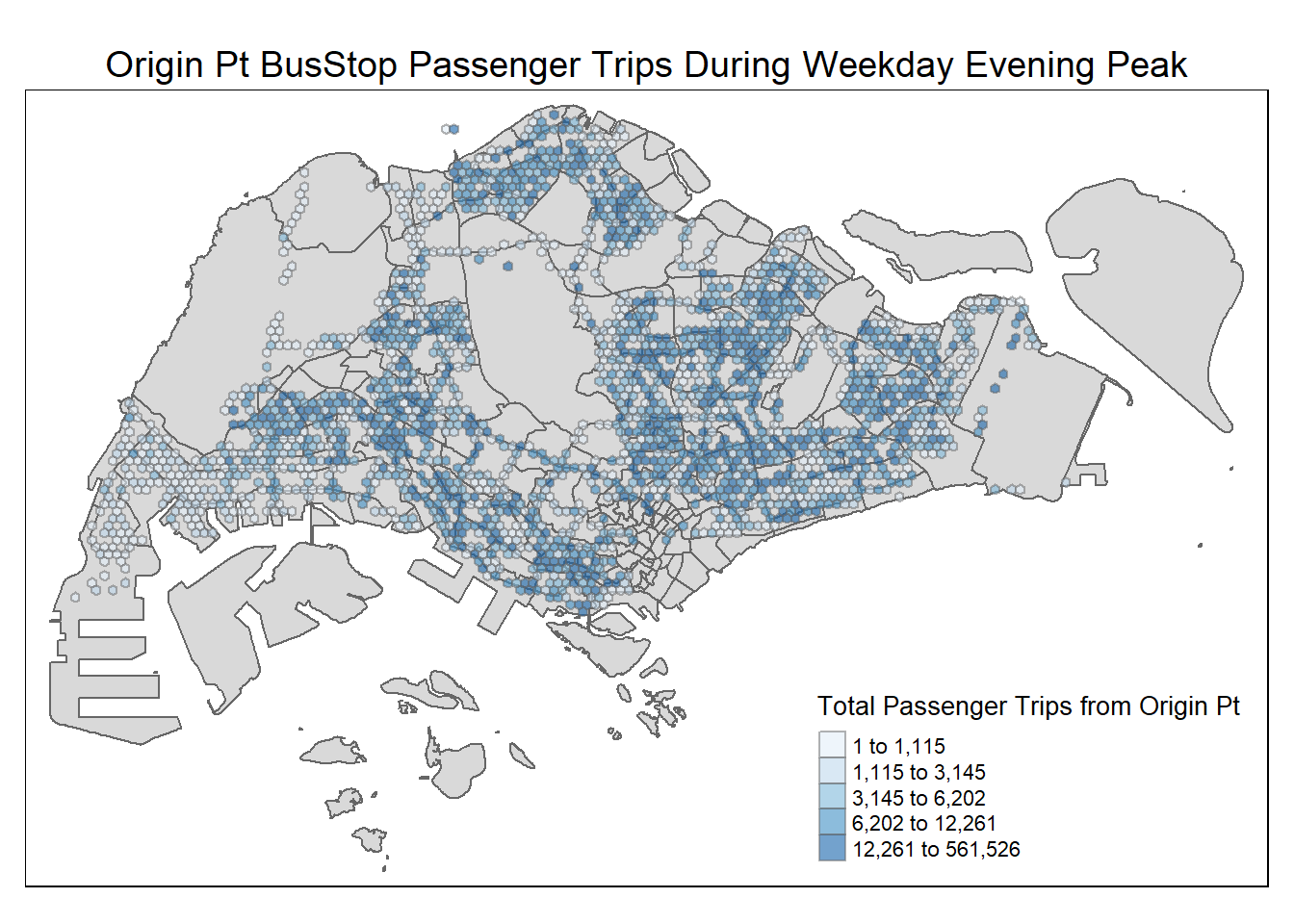

Plotting Destination Points

In order to plot the destination points, the O-D Grid data is merged with hexagon grid simple feature tibble data and filtered as follows.

wkd17_20_hxgn_grid_D_sf <- left_join(hxgn_grid_sf, 
                           wkd17_20_hxgn_grid,
                           by = c("grid_id" = "DESTIN_GRID"))%>%
  group_by(grid_id) %>%
  summarise(TOT_TRIPS = sum(TOT_TRIPS))

wkd17_20_hxgn_grid_D_sf = filter(wkd17_20_hxgn_grid_D_sf, TOT_TRIPS > 0)

The distribution of Destination points in the map is as follows.

tmap_mode("plot")

tmap mode set to plotting

tmap_options(check.and.fix = TRUE)
tm_shape(mpsz) +
  tm_polygons() +
tm_shape(wkd17_20_hxgn_grid_D_sf) +
  tm_fill(
    col = c("TOT_TRIPS"),
    palette = "Reds",
    style = "quantile",
    title = c("Total Passenger Trips from Destination Pt"),
    id = "grid_id",
    showNA = FALSE,
    alpha = 0.6,
    popup.vars = c(
      "Total Trips: " = "TOT_TRIPS"
    ),
    popup.format = list(
      TOT_TRIPS = list(format = "f", digits = 0)
    )
  ) +
  tm_layout(main.title = "Destination Pt BusStop Passenger Trips During Weekday Evening Peak",
            main.title.position = "center",
            main.title.size = 1.2,
            legend.height = 0.45, 
            legend.width = 0.35,
            frame = TRUE) +
  tm_borders(alpha = 0.5)

Warning: The shape mpsz is invalid. See sf::st_is_valid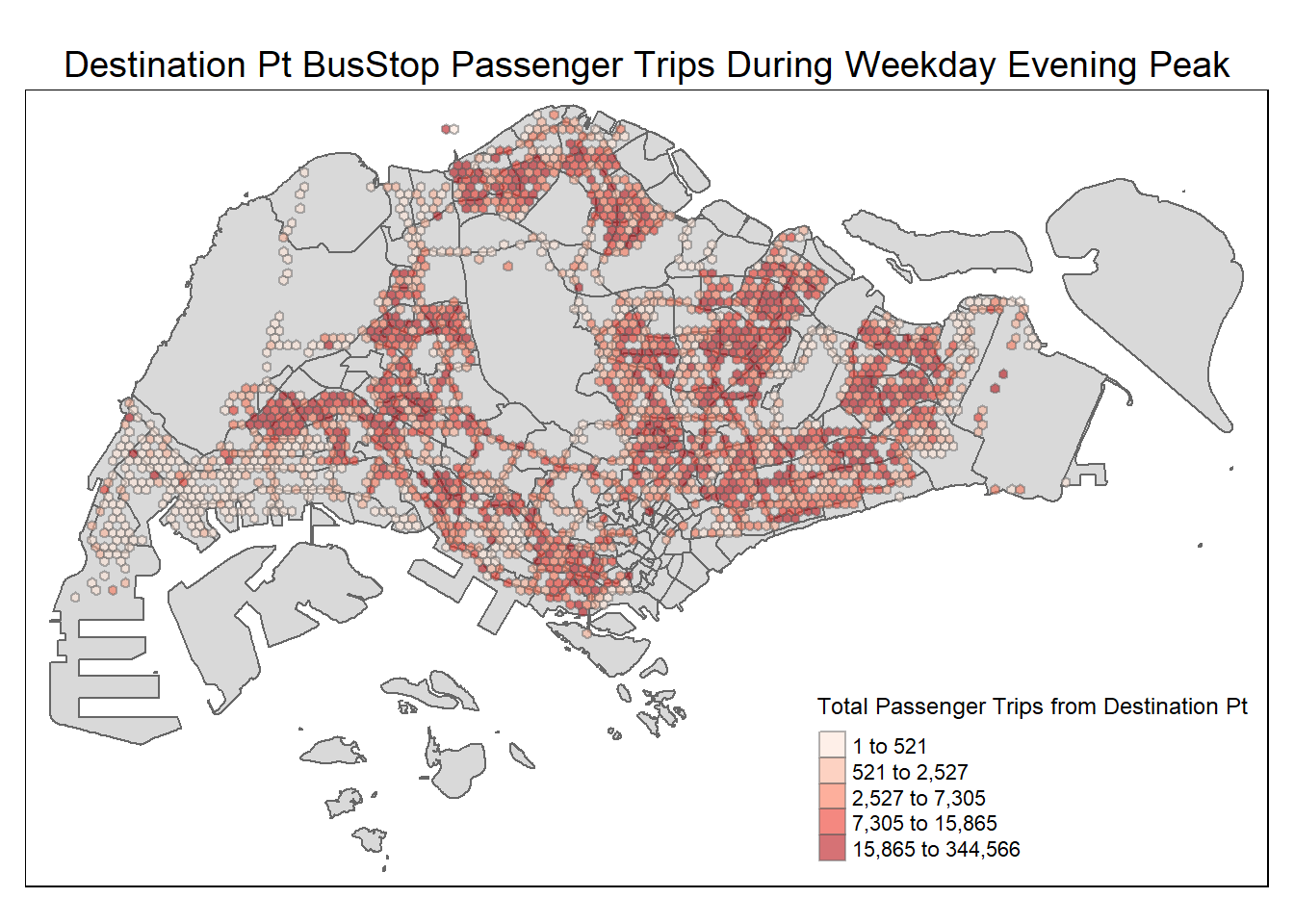

Plotting Desire lines

First the Intra-zonal flow is removed, to scope the analysis to more substantial distance of travel. Data points with Origin points same as Destination points will hence be excluded as follows.

wkd17_20_hxgn_grid_dl <- wkd17_20_hxgn_grid[wkd17_20_hxgn_grid$ORIGIN_GRID!=wkd17_20_hxgn_grid$DESTIN_GRID,]

Using od2line() function of stplanr package, the data for the desire lines are created in hexagonal grid as follows.

flowLine <- od2line(flow = wkd17_20_hxgn_grid_dl, 
                    zones = hxgn_grid_sf,
                    zone_code = "grid_id")

Creating centroids representing desire line start and end points.

To determine the appropriate ranges for a meaningful geovisualisation of the O-D desire lines, the summary statistic for the flowline is obtained as follows.

summary(flowLine)

  ORIGIN_GRID     DESTIN_GRID      TOT_TRIPS                 geometry     
 Min.   :  398   Min.   :  398   Min.   :     1.0   LINESTRING   :153812  
 1st Qu.: 5908   1st Qu.: 5880   1st Qu.:     4.0   epsg:3414    :     0  
 Median : 7753   Median : 7769   Median :    17.0   +proj=tmer...:     0  
 Mean   : 7655   Mean   : 7668   Mean   :   142.4                         
 3rd Qu.: 9315   3rd Qu.: 9324   3rd Qu.:    69.0                         
 Max.   :13258   Max.   :13258   Max.   :135939.0

From the above, there is a significant leap between the 3rd quartile to the Maximum TOT_trips. As such, a percentile close to 100% should be chosen to minimise clutter in the geovisualisation of the O-D pairs with the busiest flow. Consequently, geovisualisation of the desire lines corresponding to the top 1 percentile of TOT_trips is thus chosen for analysis, as shown below.

tm_shape(mpsz) +
  tm_polygons() +
tm_shape(busstop_hxgn_grid_sf) +
  tm_polygons() +
flowLine %>%  
  filter(TOT_TRIPS >= quantile(flowLine$TOT_TRIPS, 0.99)) %>%
tm_shape() +
  tm_lines(lwd = "TOT_TRIPS",
           style = "quantile",
           scale = c(0.1, 1, 3, 5, 7, 10),
           n = 6,
           alpha = 0.3) +
tm_layout(main.title = "Top 1% Busiest O-D flow During Weekday Evening Peak",
          main.title.position = "center",
          main.title.size = 1.1,
          legend.height = 0.4, 
          legend.width = 0.6,
          frame = TRUE)

Warning: The shape mpsz is invalid. See sf::st_is_valid

Warning in g$scale * (w_legend/maxW): longer object length is not a multiple of
shorter object length

Warning in g$scale * (x/maxW): longer object length is not a multiple of
shorter object length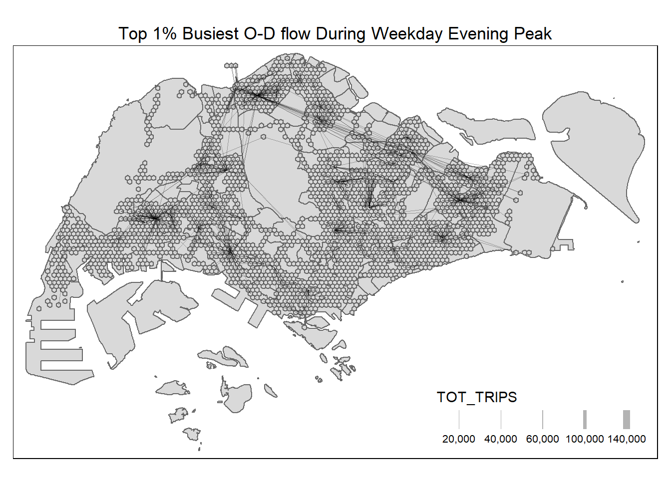

A geovisualisation of the desire lines corresponding to the median +/- 0.5 percentile of TOT_TRIPS is as shown below.

tm_shape(mpsz) +
  tm_polygons(alpha = 1, col = "red") +
tm_shape(busstop_hxgn_grid_sf) +
  tm_polygons(alpha = 1,col = "white") +
flowLine %>%  
  filter(TOT_TRIPS <= quantile(flowLine$TOT_TRIPS, 0.505),TOT_TRIPS >= quantile(flowLine$TOT_TRIPS, 0.495)) %>%
tm_shape() +
  tm_lines(lwd = "TOT_TRIPS",
           style = "quantile",
           scale = c(0.1, 1, 3, 5, 7, 10),
           n = 6,
           alpha = 0.1,
           col = "darkblue") +
tm_layout(main.title = "Median +/- 0.5 percentile of Busiest O-D flow During Weekday Evening Peak",
          main.title.position = "center",
          main.title.size = 1.1,
          legend.height = 0.4, 
          legend.width = 0.6,
          frame = TRUE)

Warning: The shape mpsz is invalid. See sf::st_is_valid

Warning in g$scale * (w_legend/maxW): longer object length is not a multiple of
shorter object length

Warning in g$scale * (x/maxW): longer object length is not a multiple of
shorter object length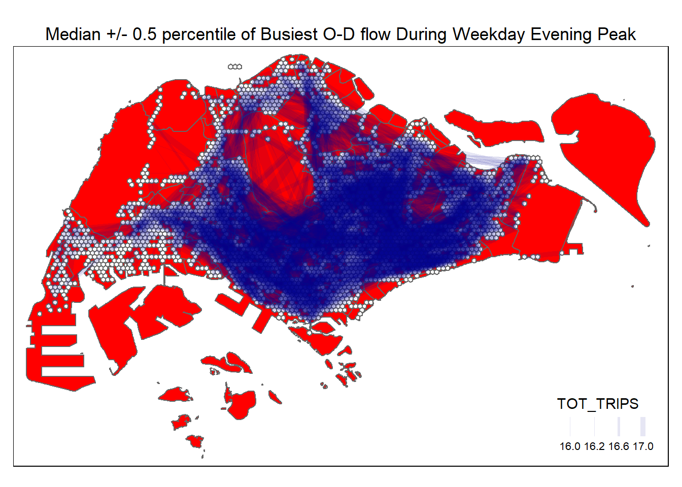

A geovisualisation of the desire lines corresponding to bottom 1 percentile of TOT_TRIPS is as shown below.

tm_shape(mpsz) +
  tm_polygons(alpha = 1, col = "red") +
tm_shape(busstop_hxgn_grid_sf) +
  tm_polygons(alpha = 1,col = "white") +
flowLine %>%  
  filter(TOT_TRIPS <= quantile(flowLine$TOT_TRIPS, 0.01)) %>%
tm_shape() +
  tm_lines(lwd = "TOT_TRIPS",
           style = "quantile",
           scale = c(0.1, 1, 3, 5, 7, 10),
           n = 6,
           alpha = 0.05,
           col = "darkblue") +
tm_layout(main.title = "Bottom 1 percentile of Busiest O-D flow During Weekday Evening Peak",
          main.title.position = "center",
          main.title.size = 1.1,
          legend.height = 0.4, 
          legend.width = 0.6,
          frame = TRUE)

Warning: The shape mpsz is invalid. See sf::st_is_valid

Warning in g$scale * (x/maxW): longer object length is not a multiple of
shorter object length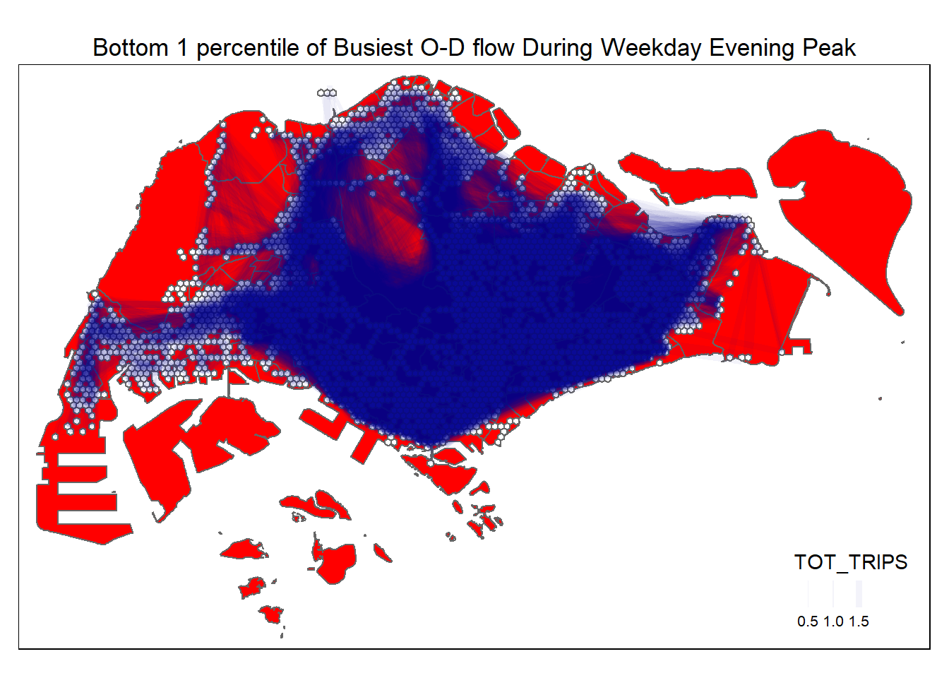

Analysis of O-D flow Geovisualisation

Identification of Propulsive and Attractiveness Variables

Computation of Distance Matrix

First as.Spatial() function of sp package will be used to convert hxgn_grid_sf from sf tibble data frame to SpatialPolygonsDataFrame (ie sp object) as follows.

busstop_hxgn_grid_sp <- as(busstop_hxgn_grid_sf, "Spatial")
busstop_hxgn_grid_sp

class       : SpatialPolygonsDataFrame 
features    : 5144 
extent      : 3605.038, 48605.04, 26249.28, 50064.98  (xmin, xmax, ymin, ymax)
crs         : +proj=tmerc +lat_0=1.36666666666667 +lon_0=103.833333333333 +k=1 +x_0=28001.642 +y_0=38744.572 +ellps=WGS84 +towgs84=0,0,0,0,0,0,0 +units=m +no_defs 
variables   : 2
names       : BUS_STOP_N, grid_id 
min values  :      01012,     398 
max values  :      99189,   13258

Next, spDists() of sp package is used to compute the Euclidean distance between the centroids of the hexagonal grid as follows.

dist <- spDists(busstop_hxgn_grid_sp, 
                longlat = FALSE)
head(dist, n=c(10, 10))

           [,1]      [,2]      [,3]      [,4]      [,5]      [,6]      [,7]
 [1,]    0.0000  992.1567 2704.1635 3333.0729  992.1567 2459.0394 2250.0000
 [2,]  992.1567    0.0000 1948.5572 2598.0762  375.0000 1634.5871 1352.0817
 [3,] 2704.1635 1948.5572    0.0000  649.5191 2281.0359  375.0000  750.0000
 [4,] 3333.0729 2598.0762  649.5191    0.0000 2928.8436  992.1567 1352.0817
 [5,]  992.1567  375.0000 2281.0359 2928.8436    0.0000 1948.5572 1634.5871
 [6,] 2459.0394 1634.5871  375.0000  992.1567 1948.5572    0.0000  375.0000
 [7,] 2250.0000 1352.0817  750.0000 1352.0817 1634.5871  375.0000    0.0000
 [8,] 2250.0000 1352.0817  750.0000 1352.0817 1634.5871  375.0000    0.0000
 [9,] 4056.2452 3269.1742 1352.0817  750.0000 3577.2720 1634.5871 1948.5572
[10,] 1634.5871  649.5191 1718.4659 2341.8742  750.0000 1352.0817  992.1567
           [,8]     [,9]     [,10]
 [1,] 2250.0000 4056.245 1634.5871
 [2,] 1352.0817 3269.174  649.5191
 [3,]  750.0000 1352.082 1718.4659
 [4,] 1352.0817  750.000 2341.8742
 [5,] 1634.5871 3577.272  750.0000
 [6,]  375.0000 1634.587 1352.0817
 [7,]    0.0000 1948.557  992.1567
 [8,]    0.0000 1948.557  992.1567
 [9,] 1948.5572    0.000 2928.8436
[10,]  992.1567 2928.844    0.0000

A list is then created, sorted according to the the distance matrix by hexagon grid id.

grid_names <- busstop_hxgn_grid_sp$grid_id

Grid_id is then attached to row and column for distance matrix matching ahead

colnames(dist) <- paste0(grid_names)
rownames(dist) <- paste0(grid_names)

The distance matrix is pivoted into a long table by using the row and column hexagon grid_id as follows.

distPair <- melt(dist) %>%
  rename(dist = value)
head(distPair, 10)

   Var1 Var2      dist
1   398  398    0.0000
2   615  398  992.1567
3   618  398 2704.1635
4   619  398 3333.0729
5   668  398  992.1567
6   671  398 2459.0394
7   725  398 2250.0000
8   725  398 2250.0000
9   728  398 4056.2452
10  777  398 1634.5871

Filtering only the non-0 distance pair to exclude intra-grid commutes and using summary(), the minimum value of the distance is obtained as follows.

distPair %>%
  filter(dist > 0) %>%
  summary()

      Var1            Var2            dist      
 Min.   :  398   Min.   :  398   Min.   :  375  
 1st Qu.: 5057   1st Qu.: 5057   1st Qu.: 7803  
 Median : 7379   Median : 7379   Median :12667  
 Mean   : 7063   Mean   : 7063   Mean   :13309  
 3rd Qu.: 9161   3rd Qu.: 9161   3rd Qu.:17863  
 Max.   :13258   Max.   :13258   Max.   :44927

An arbitrary small distance value of 0.1m is used to replace existing intra-zonal distance of 0.

distPair$dist <- ifelse(distPair$dist == 0,
                        0.1, distPair$dist)

Using summary() once more, the resultant data.frame is inspected if further wrangling is required, as follows.

distPair %>%
  summary()

      Var1            Var2            dist        
 Min.   :  398   Min.   :  398   Min.   :    0.1  
 1st Qu.: 5057   1st Qu.: 5057   1st Qu.: 7803.2  
 Median : 7379   Median : 7379   Median :12667.0  
 Mean   : 7063   Mean   : 7063   Mean   :13301.0  
 3rd Qu.: 9161   3rd Qu.: 9161   3rd Qu.:17862.8  
 Max.   :13258   Max.   :13258   Max.   :44926.5

For clarity, the origin and destination fields are renamed as follows.

distPair <- distPair %>%
  rename(orig = Var1,
         dest = Var2)

Lastly, the prepared O-D distance matrix in long form is saved as follows.

write_rds(distPair, "data/rds/distPair.rds")

Objective (2): Spatial Interaction Modelling for O-D Flows of Passengers During Weekday Evening Peakhour

Formulating Spatial Interaction Models

Preparing Flow Data & O-D attributes

Separate the intra-grid flow and from the rest of the flow data within the data.frame, and add three new fields in flow_data dataframe.

flow_data$FlowNoIntra <- ifelse( flow_data$ORIGIN_SZ == flow_data$DESTIN_SZ, 0, flow_data$TRIPS) flow_data$offset <- ifelse( flow_data$ORIGIN_SZ == flow_data$DESTIN_SZ, 0.000001, 1)